Introduction

One of the things that set statistics apart from the rest of applied mathematics is an interest in the problems introduced by sampling: how can we learn about a model if we’re given only a finite and potentially noisy sample of data?

Although frequently important, the issues introduced by sampling can be a distraction when the core difficulties you face would persist even with access to an infinite supply of noiseless data. For example, if you’re fitting a misspecified model \(m_1\) to data generated by a model \(m_2\), this misspecification will persist even as the supply of data becomes infinite. In this setting, the issues introduced by sampling can be irrelevant: it’s often more important to know whether or not the misspecified model, \(m_1\), could ever act as an acceptable approximation to the true model, \(m_2\).

Until recently, I knew very little about these sorts of issues. While reading Cosma Shalizi’s draft book, “Advanced Data Analysis from an Elementary Point of View”, I learned about the concept of pseudo-truth, which refers to the version of \(m_1\) that’s closest to \(m_2\). Under model misspecification, estimation procedures often converge to the pseudo-truth as \(n \to \infty\).

Thinking about the issues raised by using a pseudo-true model rather than the true model has gotten me interested in learning more about quantifying approximation error. Although I haven’t yet learned much about the classical theory of approximations, it’s clear that a framework based on approximation errors allows one to formalize issues that would otherwise require some hand-waving.

A General Framework for Quantifying Approximation Error

Suppose that I want to approximate a function \(f(x)\) with another function \(g(x)\) that comes from a restricted set of functions, \(G\). What does the optimal approximation look like when \(g(x)\) comes from a parametric class of functions \(G = {g(x, \theta) \lvert \theta \in \mathbb{R}^{p}}\)?

To answer this question with a single number, I think that one natural approach looks like:

1. Pick a point-wise loss function, \(L(f(x), g(x))\), that evaluates the gap between \(f(x)\) and \(g(x)\) at any point \(x\).
2. Pick a set, \(S\), of values of \(x\) over which you want to evaluate this point-wise loss function.
3. Pick an aggregation function, \(A\), that summarizes all of the point-wise losses incurred by any particular approximation \(g(x, \theta)\) over the set \(S\).

Given \(L\), \(S\) and \(A\), you can define an optimal approximation from \(G\) to be a function, \(g \in G\), that minimizes the aggregated point-wise loss function over all values in \(S\).

An Analytically Tractable Special Case

This framework is so general that I find it hard to reason about. Let’s make some simplifying assumptions so that we can work through an analytically tractable special case:

1. Let’s assume that \(f(x) = x^2\). Now we’re trying to find the optimal approximation of a quadratic function.
2. Let’s assume that \(g(x, \theta) = g(x, a, b) = ax + b\), where \(\theta = \langle a, b \rangle \in \mathbb{R}^{2}\). Now we’re trying to find the optimal linear approximation to the quadratic function, \(f(x) = x^2\).
3. Let’s assume that the point-wise loss function is \(L(f(x), g(x, \theta)) = [f(x) - g(x, \theta)]^2\). Now we’re quantifying the point-wise error using the squared error loss that’s commonly used in linear regression problems.
4. Let’s assume that \(S\) is a closed interval on the real line, that is \(S = [l, u]\).
5. Let’s assume that the aggregation function, \(A\), is the integral of the loss function, \(L\), over the interval, \([l, u]\).

Under these assumptions, the optimal approximation to \(f(x)\) from the parametric family \(g(x, \theta)\) is defined as a solution, \(\theta^{*}\), to the following minimization problem:

$$ \begin{align*} \theta^{*} &= \arg \min_{\theta} \int_{l}^{u} L(f(x), g(x, \theta)) dx \
&= \arg \min_{\theta} \int_{l}^{u} [f(x) - g(x, \theta)]^2 dx \
&= \arg \min_{\theta} \int_{l}^{u} [x^2 - (ax + b)]^2 dx \
\end{align*}. $$

I believe that this optimization problem describes the pseudo-truth towards which OLS univariate regression converges when the values of the covariate, \(x\), are drawn from a uniform distribution over the interval \([l, u]\). Simulations agree with this belief, although I may be missing some important caveats.

Solving the Problem Analytically

To get a feeling for how the pseudo-truth behaves in this example problem, I found it useful to solve for the optimal linear approximation analytically by computing the gradient of the cost function with respect to \(\theta\) and then solving for the roots of the resulting equations:

$$ \frac{\partial}{\partial a} \int_{l}^{u} [x^2 - (ax + b)]^2 dx = 0 \
\frac{\partial}{\partial b} \int_{l}^{u} [x^2 - (ax + b)]^2 dx = 0 \
$$

After some simplification, this reduces to a matrix equation:

$$ \begin{bmatrix} \frac{2}{3} (u^3 - l^3) & u^2 - l^2 \
u^2 - l^2 & 2 (u - l) \
\end{bmatrix} \begin{bmatrix} a \
b \
\end{bmatrix} = \begin{bmatrix} \frac{1}{2} (u^4 - l^4) \
\frac{2}{3} (u^3 - l^3) \
\end{bmatrix}. $$

In practice, I suspect it’s much easier to solve for the optimal approximation on a computer by using quadrature to approximate the aggregated point-wise loss function and then minimizing that aggregation function using a quasi-Newton method. I experimented a bit with this computational approach and found that it reproduces the analytic solution for this problem. The computational approach generalizes to other problems readily and requires much less work to get something running.

Some Optimal Linear Approximations to a Quadratic Function over Different Intervals

You can see examples of the pseudo-truth versus the truth below for a few intervals \([l, u]\):

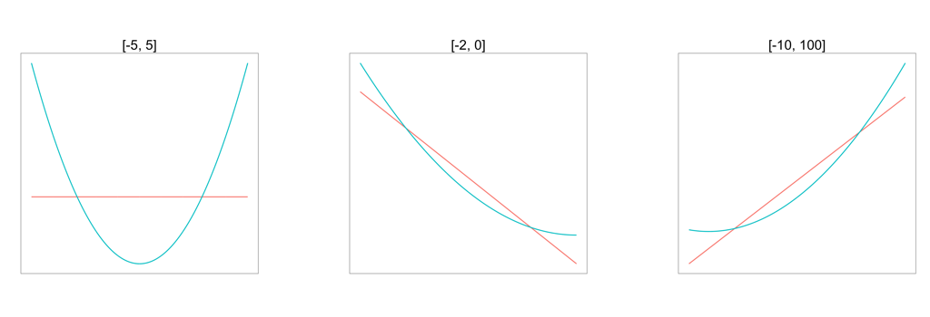
I don’t think there’s anything very surprising in these plots, but I nevertheless find the plots useful for reminding myself how sensitive the optimal approximation is to the set \(S\) over which it will be applied.

Formally Defining Asymptotic Bias

One reason that I find it useful to think formally about the quality of optimal approximations is that it makes it easier to rigorously define some of the problems that arise in machine learning.

Consider, for example, the issues raised in this blog post by Paul Mineiro:

In statistics the bias-variance tradeoff is a core concept. Roughly speaking, bias is how well the best hypothesis in your hypothesis class would perform in reality, whereas variance is how much performance degradation is introduced from having finite training data.

I would say that this definition of bias is quite far removed from the definition used in statistics and econometrics, although it can be formalized in terms of the expected point-wise loss.

The core issue, as I see it, is that, for a statistician or econometrician, bias is not an asymptotic property of a model class, but rather a finite-sample property of an estimator. Variance is also a finite-sample property of an estimator. Some estimators, such as the ridge estimator for a linear regression model, decrease variance by increasing bias, which induces a trade-off between bias and variance in finite samples.

But Paul Mineiro is not, I think, interested in these finite-sample properties of estimators. I believe he’s concerned about the intrinsic error introduced by approximating one function with another. And that’s a very important topic that I haven’t seen discussed as often as I’d like.

Put another way, I think Mineiro’s concern is much more closely linked to formalizing an analogue for regression problems of the concepts of VC dimension and Rademacher complexity that come up in classification problems. Because I wasn’t familiar with any such tools, I found it helpful to work through some problems on optimal approximations. Given this framework, I think it’s easy to replace Mineiro’s concept of bias with an approximation error formalism that might be called asymptotic bias or definitional bias, as Efron does in this paper. These tools let one quantify the costs incurred by the use of a pseudo-true model rather than the true model.

I’d love to learn more about this issue. As it stands, I know too much about sampling and too little about quantifying the quality of approximations.